Once you’ve worked through the foundational Desmos techniques (linear regression, sliders, graphing systems, the percent and fraction shortcuts), you’ve got the core toolkit most students rely on. (If you haven’t yet, start with the free Ten Tips for Desmos on the Digital SAT guide before going further.)
This post is what comes next. Below are ten advanced Desmos techniques that go beyond the basics. The point is speed: fewer algebra slips, fewer long setups, and more time for the questions that actually require thinking.
Every technique here can be practiced at desmos.com/practice, but you should also try them inside Bluebook, since that is the actual SAT testing environment. Confirming a trick works there is the only way to be sure you can rely on it on test day.
One thing worth saying up front: the goal here is not to avoid math entirely. Desmos earns its place when it is genuinely faster or less error-prone than working by hand. When the algebra is just as quick (a one-step substitution, a simple factorization), doing it by hand is often faster than opening the calculator at all.
1. Solve Any Equation by Graphing Both Sides
This is one of the most useful shortcuts on the Digital SAT. Instead of solving algebraically (which can get ugly with radicals, exponentials, absolute values, or rational expressions), type the left side as one equation and the right side as another, then read off the intersection.
Example: If 2x = x + 4, what are the approximate solutions?
Solution: Enter y = 2x and y = x + 4 as two separate lines. Click the gray dots that appear at each intersection.
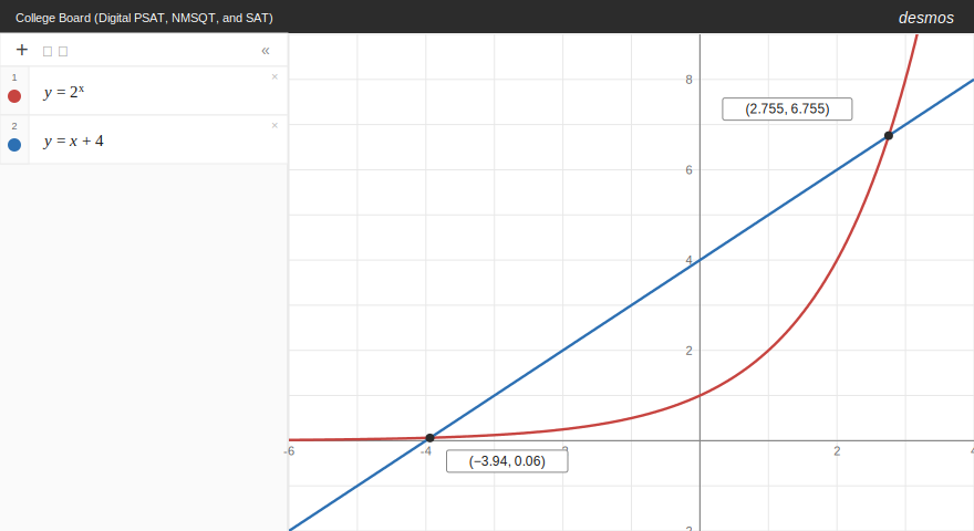
The two curves cross at approximately (−3.94, 0.06) and (2.755, 6.755), so the solutions are x ≈ −3.94 and x ≈ 2.755. Faster and less error-prone than algebraic manipulation.
Use this approach any time you see an equation that mixes function types: quadratic equals linear, exponential equals polynomial, square root equals rational. Set each side to y, graph both, intersect.
2. Quadratic Regression for Table Problems
Linear regression is the basic version of this technique, but Desmos can also fit quadratics, exponentials, and several other curve types, and it is easier than you might expect. The trick is the regression dropdown that appears once you have entered table data.
Example: The table below shows values of a function. What is the value of f(7)?
| x | f(x) |
|---|---|
| 1 | 5 |
| 2 | 11 |
| 3 | 19 |
| 4 | 29 |
Solution: Enter the four points into a Desmos table. Click the small regression icon (the dark circle with the curve and dots) on the upper-left of the table panel. A dropdown appears letting you choose Linear Regression, Quadratic Regression, Exponential Regression, and several others. Select Quadratic Regression.
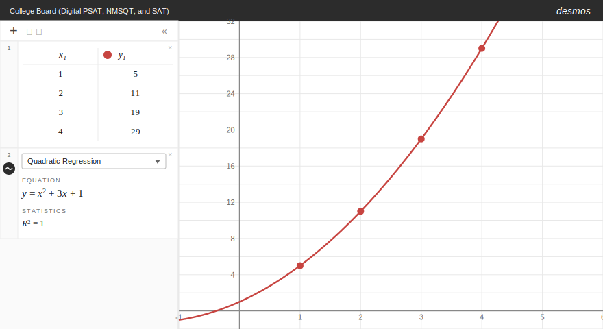
Desmos returns y = x2 + 3x + 1 with R2 = 1 (a perfect fit, as expected). Plug in x = 7: f(7) = 49 + 21 + 1 = 71.
This dropdown is much faster than typing out the regression syntax, and the R2 value tells you immediately how good the fit is, which is useful when you are not sure which curve type to choose.
Important: the regression dropdown is a Desmos feature, not guaranteed in Bluebook. Always test this in the official Bluebook app before relying on it. If it’s unavailable, use regression syntax instead (y₁ ~ ax₁2 + bx₁ + c for a quadratic fit).
3. Exponential Regression for Growth and Decay
Same dropdown, different option. Use Exponential Regression any time the data shows multiplicative growth or decay: compound interest, populations, depreciation, half-life problems.
Example: A bacterial culture is measured each hour, with the populations shown below. If the pattern continues, what will the population be at hour 10?
| Hour | Population |
|---|---|
| 0 | 200 |
| 1 | 240 |
| 2 | 288 |
| 3 | 346 |
| 4 | 415 |
Solution: Enter the data into a table, click the regression icon, and choose Exponential Regression.
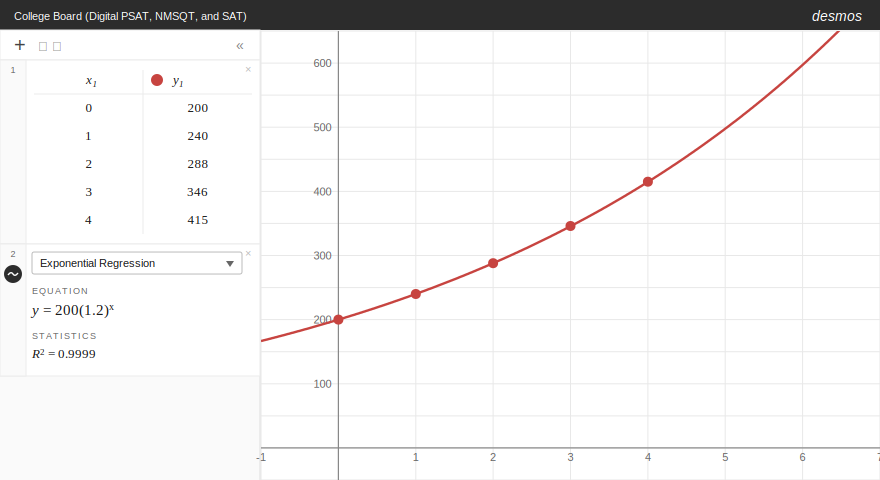
Because the table values are rounded, the regression will not return exact parameters, but it clearly indicates an initial population near 200 and a growth factor near 1.2. So the underlying model is approximately y = 200(1.2)x, and at hour 10 the model predicts a population of approximately 200(1.2)10 ≈ 1,238.
If you are ever unsure whether data is linear, quadratic, or exponential, try each regression type and compare the R2 values. Use R2 as a clue, but also check that the model type makes sense for the situation. Population growth, compound interest, and decay problems are exponential by nature, while data with a clear “turning point” is usually quadratic.
4. Define Functions to Reuse Throughout a Problem
Most students retype expressions every time they need to evaluate one. Instead, define the function once and Desmos will let you call it as many times as you want. This pays off enormously on multi-part problems and on questions involving function composition.
Example: If f(x) = 2x2 − 3x + 5, what is the value of f(f(2))?
Solution: Type f(x) = 2x2 − 3x + 5 in line 1. Now you can evaluate the function at any input, and Desmos shows the result immediately.
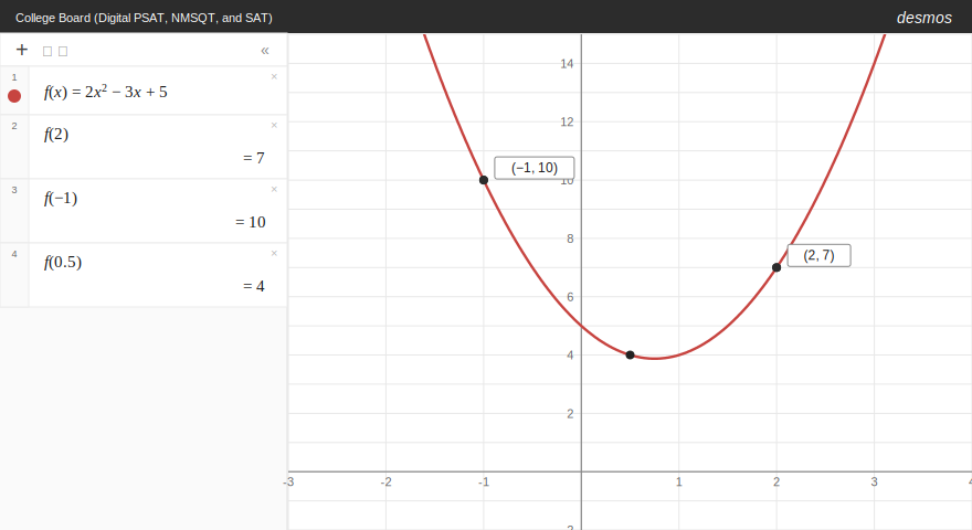
From the panel, f(2) = 7. Now type f(7) to get the second composition: f(7) = 2(49) − 21 + 5 = 82. So f(f(2)) = 82.
This technique is especially powerful when a problem references the same complicated expression multiple times, for example in word problems where a revenue or cost function gets evaluated at several different production levels.
5. Use Lists to Test All the Answer Choices at Once
This trick can save real time on hard multiple-choice questions. Once you’ve defined a function (Tip 4), you can pass it a list of inputs in square brackets, and Desmos will return a list of outputs.
Example: Which of the following is a solution to x2 − 5x + 6 = 0?
(A) 1 (B) 2 (C) 4 (D) 5
Solution: Define f(x) = x2 − 5x + 6, then evaluate f([1, 2, 4, 5]).
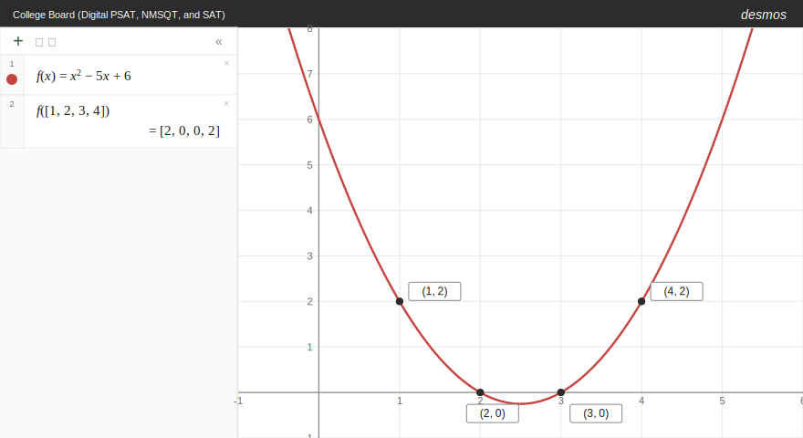
Desmos returns [2, 0, 2, 6]. The second entry is zero, so x = 2 is the solution. The answer is B.
This works for any problem where you can plug each answer choice into a single expression: “which value satisfies this equation,” “which point lies on the graph,” “which input gives the maximum output.” Bundle them into a list and you are done in one keystroke. (For more practice on these question types, the SAT math drills have plenty of multiple-choice problems where this approach really pays off.)
6. Restrict the Domain with Curly Braces
Adding {condition} after a function tells Desmos to only graph the function where the condition is true. This is useful for visualizing piecewise functions, graphing only the relevant portion of a curve, or quickly checking the behavior of a function over a specific interval.
Example: What is the range of f(x) = x2 when x < 0?
Solution: Type y = x2 {x < 0} into Desmos.
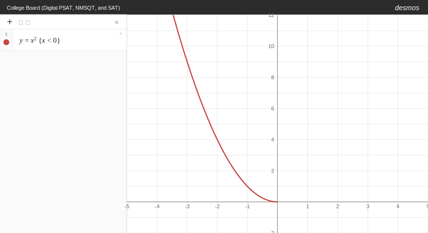
You see only the left half of the parabola. As x approaches 0 from the left, y approaches 0; as x moves toward negative infinity, y grows without bound. The range is y > 0.
You can also chain conditions, like {−2 ≤ x ≤ 5}, to graph a function on a closed interval. (Use the ≤ and ≥ symbols from the Desmos keyboard for closed endpoints, or strict < and > for open ones.) This is the cleanest way to handle piecewise definitions on Digital SAT questions.
7. Find All Real Zeros of a Polynomial by Graphing
The Digital SAT regularly asks about zeros, x-intercepts, and “how many real solutions” of polynomial equations, and not just for quadratics. For cubics, factored polynomials, and higher-degree expressions, graphing is far faster than algebraic factoring. Plot the function and read off the zeros from the gray dots that appear where the curve touches or crosses the x-axis.
Example: How many real solutions does x3 − 4x2 + x + 6 = 0 have, and what are they?
Solution: Type y = x3 − 4x2 + x + 6 into Desmos and look at where the curve touches or crosses the x-axis.
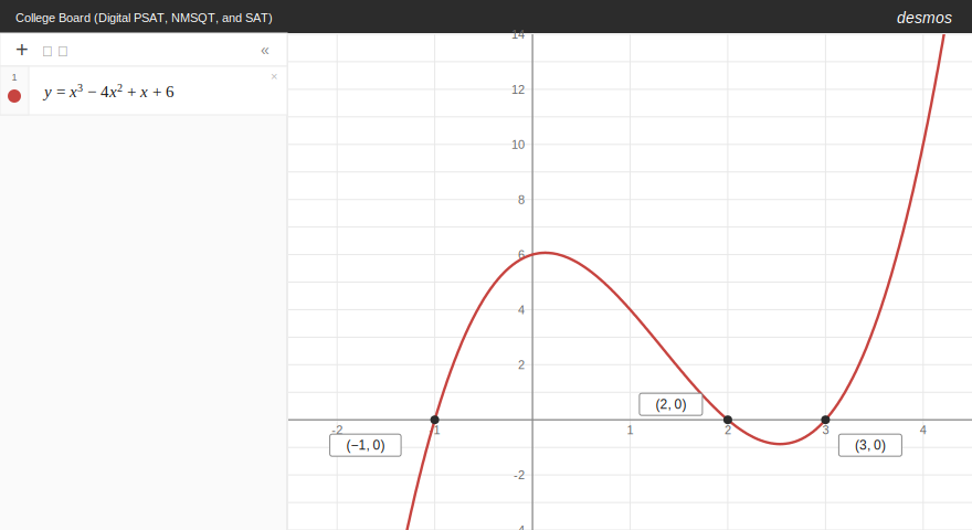
The cubic crosses the x-axis at three points: x = −1, 2, and 3. So there are three real solutions. (As a sanity check, the polynomial factors as (x + 1)(x − 2)(x − 3); graphing made that visible without doing any factoring.)
This technique is especially useful when a polynomial doesn’t factor cleanly. The SAT will sometimes give you a cubic with one rational zero and two irrational ones, and graphing lets you see all three at a glance even when the algebra is messy.
8. Verify Equivalent Expressions by Graphing
“Which of the following is equivalent to…” is one of the most common Digital SAT Advanced Math question types, and one of the easiest to mess up by hand because of sign errors when you expand or factor. Desmos gives you a strong visual check: graph the original expression and each answer choice on separate lines. The one whose graph perfectly overlays the original is the equivalent expression.
Example: Which of the following is equivalent to (x + 3)2 − 9?
(A) x2 + 6x (B) x2 + 9 (C) x2 − 9 (D) x2 + 6x + 9
Solution: Type y = (x + 3)2 − 9 on line 1. Then test each answer choice on subsequent lines. Choice (A), y = x2 + 6x, draws the exact same parabola; its graph lies directly on top of the original.
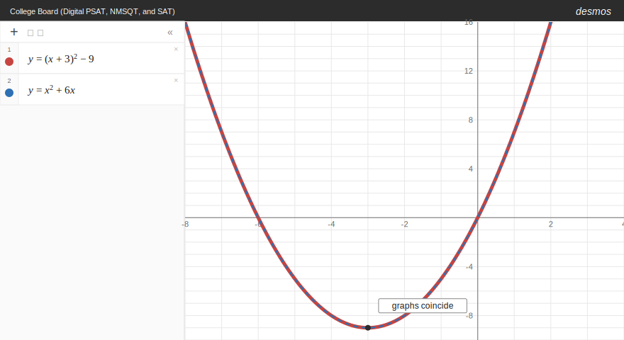
The two graphs coincide perfectly, so (x + 3)2 − 9 = x2 + 6x. The answer is A. (You can verify algebraically: (x + 3)2 − 9 = x2 + 6x + 9 − 9 = x2 + 6x.)
For most SAT-style polynomial expressions, matching graphs reliably indicate equivalence. For rational expressions, also check a few specific x-values, since holes or domain restrictions may not be visible at default zoom.
Pro tip: if multiple answer choices look close to the original on the graph, zoom in. Even a small constant difference will be visible at a tighter zoom level.
9. Solve Polynomial Inequalities by Graphing
Inequality questions on the Digital SAT often ask “for what values of x is f(x) ≥ 0?” or similar. The algebraic approach (factoring, sign-charting, considering each region) is error-prone. Graphing is much cleaner: the inequality f(x) ≥ 0 is true for x-values where the graph lies on or above the x-axis, and f(x) ≤ 0 for x-values where it lies on or below.
Example: What is the solution set to (x − 1)(x − 4) ≤ 0?
Solution: Graph y = (x − 1)(x − 4) in Desmos and identify the region where the curve is at or below the x-axis.
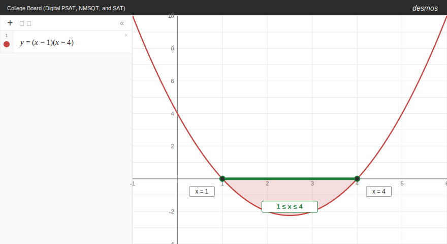
The parabola dips below the x-axis between its two zeros, x = 1 and x = 4. So the solution is 1 ≤ x ≤ 4.
This approach generalizes to higher-degree polynomials and rational expressions. For something like x3 − 4x ≥ 0, graph it and read off the intervals where the curve is on or above the x-axis. The key is just remembering: above the x-axis = positive, below = negative, on the axis = zero. Strict inequalities (< or >) exclude the zeros; non-strict inequalities (≤ or ≥) include them.
10. Use Two Sliders for Two-Unknown Problems
You probably already use sliders for problems with one unknown constant. Sliders compose: type any equation with two unknown letters, and Desmos creates a slider for each. They are best used as an exploration tool, to see what kinds of values produce the right behavior, rather than as the primary way to find a precise answer.
Example: The graph of y = ax2 + bx − 6 passes through the points (1, −5) and (3, 9). What are the values of a and b?
Solution: Type y = ax2 + bx − 6 into Desmos. You’ll be prompted to add sliders for both a and b. Also plot the two reference points by typing (1, −5) and (3, 9) on separate lines.
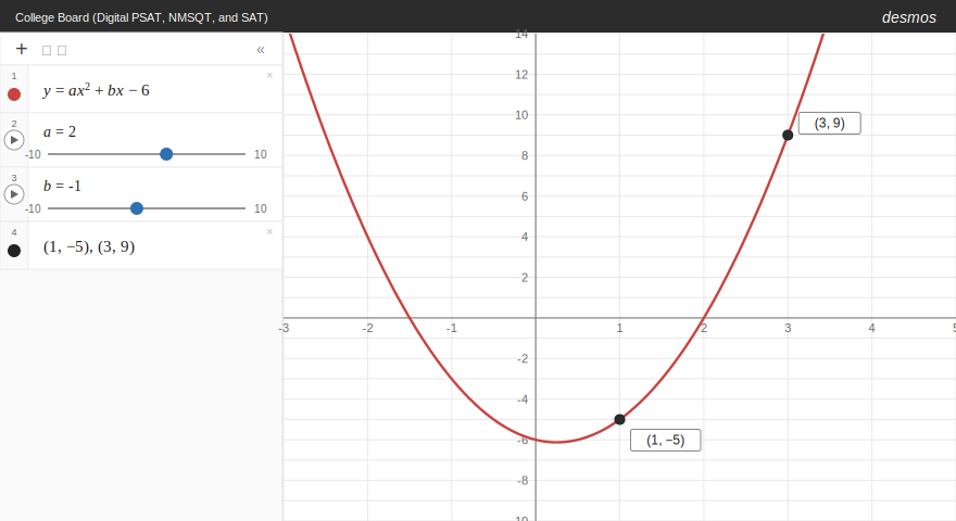
Drag the sliders to get a feel for how each parameter changes the parabola, which helps you sanity-check your answer. But for the precise values, the algebra is faster. Substituting (1, −5) and (3, 9) into y = ax2 + bx − 6 gives:
a + b = 1
9a + 3b = 15
Solving the system gives a = 2, b = −1. You can then type those exact values directly into the slider boxes (click on the slider’s number, type in the value) and confirm the parabola passes through both points.
The same workflow applies to any “find two unknown coefficients” problem: quadratic identities, systems with two unknown constants, or “for what values does the equation pass through these points” questions. Use sliders to explore and verify; use the algebra to find the exact answer.
Tip: if you do want to use sliders alone for a final answer, change the step size first. The default is 1; change it to 0.1 or 0.01 (click the slider’s gear icon) for finer control.
Putting It All Together
None of these techniques replaces conceptual math knowledge. Desmos can compute a regression in two seconds, but you still have to recognize when a problem calls for one. The students who improve fastest pair fluent Desmos technique with strong underlying algebra and an eye for when each tool applies.
The best way to build that fluency is to drill problems where you actively choose between approaches. Try these techniques on real, timed Digital SAT math questions, like the practice drills in our SAT math drill library, and watch your section times come down.
The fastest SAT math students know exactly when to skip the algebra and reach for the calculator instead.
SAT® and PSAT/NMSQT® are registered trademarks of the College Board. Desmos® is a trademark of Desmos Studio PBC. This content is not affiliated with or endorsed by the College Board or Desmos Studio.